Enunciado
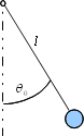
El movimiento de un péndulo simple sin fricción que empieza a oscilar en $\theta=\theta_0$ se describe mediente el siguiente problema de valor inicial:
$$\hspace{3cm}\frac{d^2\theta}{d\tau ^2}+\frac{g}{l}\,\mbox{sen}\, \theta=0 \hspace{.5cm} ,\hspace{.5cm} \theta(0)=\theta_0 \hspace{.5cm} ,\hspace{.5cm} \frac{d\theta}{d\tau}(0)=0\hspace{3cm}$$
donde se ha llamado
|
 |
- Busca una variable temporal, $t$, para la cual la ecuación anterior no tenga parámetros.
- Utiliza la nueva ecuación para representar una estimación del movimiento y de la velocidad cuando la variable $t$ varía entre $0$ y $10$, tomando tres valores diferentes de $\theta_0$ (siempre entre $0$ y $\pi$ ambos excluidos). Realiza una gráfica con las tres estimaciones del ángulo en función de $t$ y otra con las tres estimaciones de la velocidad.
Resolución del primer apartado
Planteamos un cambio de variable de la forma
$$t=c\tau$$
y hemos de hallar el valor de $c$ tal que la ecuación diferencial para $\theta$ y $t$ no tenga parámetros. Para ello empezamos escribiendo las derivadas de $\theta$ respecto de $\tau$ en función de las derivadas de $\theta$ respecto de $t$. Hazlo tú y pulsa en 'Ver'.
Ver
$$t=c\tau \hspace{.5cm} \Rightarrow \hspace{.5cm} \frac{d\theta}{d\tau}=c\frac{d\theta}{dt}
\hspace{.5cm} \Rightarrow \hspace{.5cm} \frac{d^2\theta}{d\tau^2}=c^2\frac{d^2\theta}{dt^2}$$
Ahora sustituimos en la ecuación diferencial,
$$\frac{d^2\theta}{d\tau ^2}+\frac{g}{l}\,\mbox{sen}\, \theta=0
\hspace{.5cm} \Rightarrow \hspace{.5cm} c^2\frac{d^2\theta}{dt^2}+\frac{g}{l}\,\mbox{sen}\, \theta=0$$
Si queremos que esta última ecuación no tenga parámetros, debemos forzar que
$$\frac{g}{l}=c^2$$
de donde $$c=\sqrt{\frac{g}{l}}$$
La nueva variable es $$t=\sqrt{\frac{g}{l}} \tau$$ y el nuevo problema de valor inicial es entonces ... escríbelo y pulsa en 'Continuar'.
Con el cambio $t=\sqrt{\frac{g}{l}} \tau$, el problema de valor inicial es
$$\frac{d^2\theta}{dt^2}+\mbox{sen}\, \theta=0 \hspace{.5cm} , \hspace{.5cm} \theta(0)=\theta_0
\hspace{.5cm} , \hspace{.5cm} \frac{d\theta}{dt}(0)=0$$
Debe observarse que la nueva variable, $t$, es adimensional puesto que $\sqrt{\frac{g}{l}}$ tiene unidades de $1/\mbox{Tiempo}$.
Resolución del segundo apartado
Como en otros problemas, utilizaremos el comando 'ode45' para aproximar la solución del sistema equivalente al problema de valor inicial anterior. Escribe el sistema y pulsa en 'Ver'.
Ver
En este caso el sistema diferencial de primer orden equivalente al p.v.i. es
$$\left\{\begin{array}{lll}x'_1(t)=x_2(t) & , & x_1(0)=\theta_0 \\ x'_2(t)=-\mbox{sen}\, x_1(t) & , & x_2(0)=0 \end{array}\right.$$
donde $x_1(t)=\theta(t)$ y $x_2(t)=\theta'(t)$.
Preparamos a continuación el código para
- Calcular las estimaciones de $x_1$ y $x_2$ utilizando 'ode45'; tomaremos las tres condiciones iniciales siguientes: $$\theta_0=\frac{\pi}{8} \hspace{.5cm}, \hspace{.5cm} \theta_0=\frac{\pi}{4} \hspace{.5cm}, \hspace{.5cm} \theta_0=\frac{\pi}{2}$$ y un vector de valores de dimensión 50 en la variable $t$.
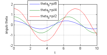
- En la figura 1 se representarán las tres estimaciones para $x_1$, añadiéndoles etiquetas a los ejes y una leyenda con los valores iniciales de cada gráfica
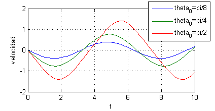
- En la figura 2 haremos la propio con las velocidades
f=@(t,x) [x(2); -sin(x(1))];
vt=linspace(0,10,50);
[t,xest1]=ode45(f,vt,[pi/8 0]);
[t,xest2]=ode45(f,vt,[pi/4 0]);
[t,xest3]=ode45(f,vt,[pi/2 0]);
figure(1)
plot(t,xest1(:,1),t,xest2(:,1),t,xest3(:,1))
legend('theta_0=pi/8','theta_0=pi/4','theta_0=pi/2')
xlabel('t');ylabel('ángulo theta')
grid on
figure(2)
plot(t,xest1(:,2),t,xest2(:,2),t,xest3(:,2))
legend('theta_0=pi/8','theta_0=pi/4','theta_0=pi/2')
xlabel('t');ylabel('velocidad')
grid on
Ejecuntando estas líneas obtendremos en la figura 1 las gráficas de las aproximaciones del ángulo (el cuadro con la leyenda se ha movido posteriormente):